Dense Depth Summer Research (DDSR2020)

We trained a model predict a depth value for every pixel of a given image. This page is an adapted README from the GitHub repo, which you can find here.

Description

Over the summer of 2020, I worked in a group (consisting of four people) to ultimately create a system of deep convolutional neural networks to estimate the depth values (distance from the camera) of all pixels in a given image. You can find examples of our task below. The group effort consisted primarily of Alex Jiang and I, with help from Kevin Shen and Aaron Marmolejos. The group was mentored by Quinn Shen.

We implemented the research of Monodepth2 - Digging into Self-Supervised Monocular Depth Prediction (ICCV 2019) and explored extensions to this research. We found that replacing the original residual neural network (ResNet) encoder with a densely connected convoluational network (DenseNet) encoder resulted in better quantitative metrics (how “accurate” the model is) and faster model covergence. We observed that for similar levels of accuracy in dense depth, the DenseNet architecture is more efficient in number of learned parameters and computation at the trade-off of memory usage during training.

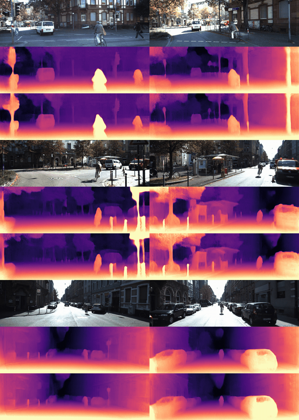
An example scene from the KITTI dataset. Top: Original input image | Middle: Baseline Monodepth2 (ResNet-18) | Bottom: DenseNet-121

Metrics & Pre-Trained Model Checkpoints

KITTI Eigen Dataset (LiDAR ground truth)

We evaluate our models on 7 quantitative metrics: absolute relative error, squared relative error, root mean squared error, root mean squared log error, and accuracy under selected thresholds (\(1.25 \%\), \(1.25^2 \%\), \(1.25^3 \%\)).

Below is a quick explanation of how the metrics are calculated. \(\hat{d}\) is the predicted depth value for a pixel and \(d\) is the ground truth depth value of that pixel.

Absolute relative error:
\[\frac 1 n \sum \frac{| \hat{d} - d |}{d}\]
Squared relative error:
\[\frac 1 n \sum \frac{ (\hat{d} - d )^2 }{d}\]
Root mean squared error:
\[\sqrt{\frac 1 n \sum (\hat{d} - d)^2 }\]
Root mean squared log error:
\[\sqrt{\frac 1 n \sum (\log \hat{d} - \log d)^2}\]
Accuracy under threshold:

Percentage of depth values \(d\) fulfilling: \(\max \left(\frac{\hat d}{d}, \frac{d}{\hat d} \right) < \text{threshold}\)

For all error metrics, lower is better. For all accuracy metrics, higher is better. The best values are bolded. The Mono (M), Stereo (S), and Mono + Stereo (MS) training modes are separated for comparison.

Model Name	abs_rel	sq_rel	rmse	rmse_log	a1	a2	a3
Baseline (M)	0.119	0.935	4.938	0.196	0.868	0.958	0.981
DenseNet (M)	0.107	0.794	4.564	0.182	0.890	0.965	0.983

Model Name	abs_rel	sq_rel	rmse	rmse_log	a1	a2	a3
Baseline (S)	0.108	0.832	4.858	0.202	0.866	0.952	0.977
DenseNet (S)	0.103	0.807	4.803	0.199	0.876	0.954	0.978

Model Name	abs_rel	sq_rel	rmse	rmse_log	a1	a2	a3
Baseline (MS)	0.103	0.793	4.690	0.190	0.878	0.960	0.981
DenseNet (MS)	0.098	0.705	4.445	0.185	0.888	0.962	0.982

Note: All models were trained with an image resolution of 1024 x 320. (Full metrics spreadsheet can be found here.)

Memory Usage & Inference Speed

	ResNet18 (MS)	DenseNet121 (MS)
Reserved Memory	1.79GB	2.52GB
Avg. Inference Speed	11.0ms	45.4ms

Note: Inference speed was measured on a GTX 1050 Ti GPU on 1024 x 320 images. (Full memory usage and inference speed metrics here.)

Qualitative Evaluation

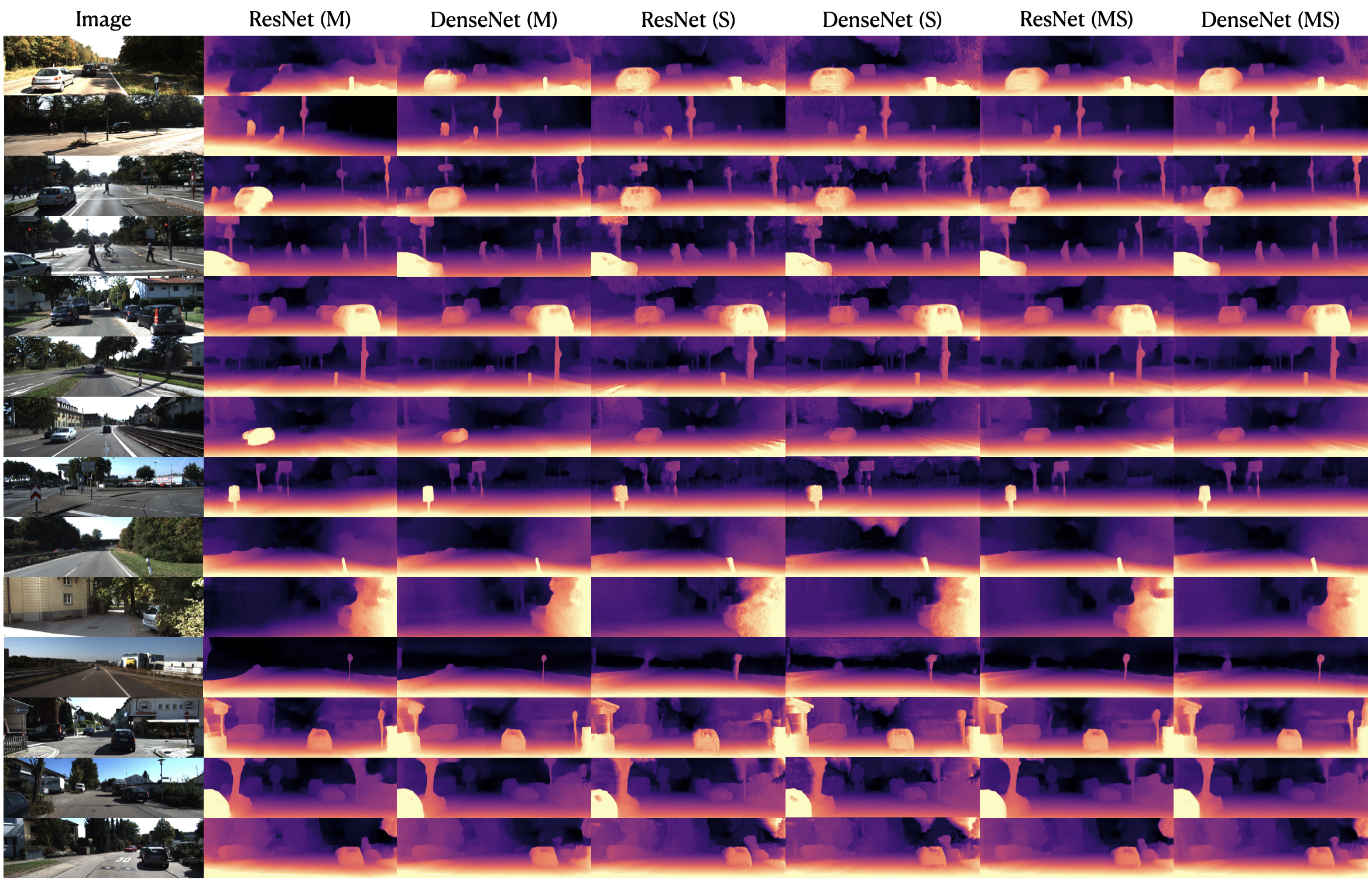
Here are some qualitative results comparing Monodepth2 ResNet-18 vs. DenseNet-121 models side-by-side from manually-curated KITTI scenes. Mono, Stereo, and Mono + Stereo are grouped together for easy side-by-side comparison.

Qualitative comparison of ResNet-18 and DenseNet-121

TensorBoard Visualizations

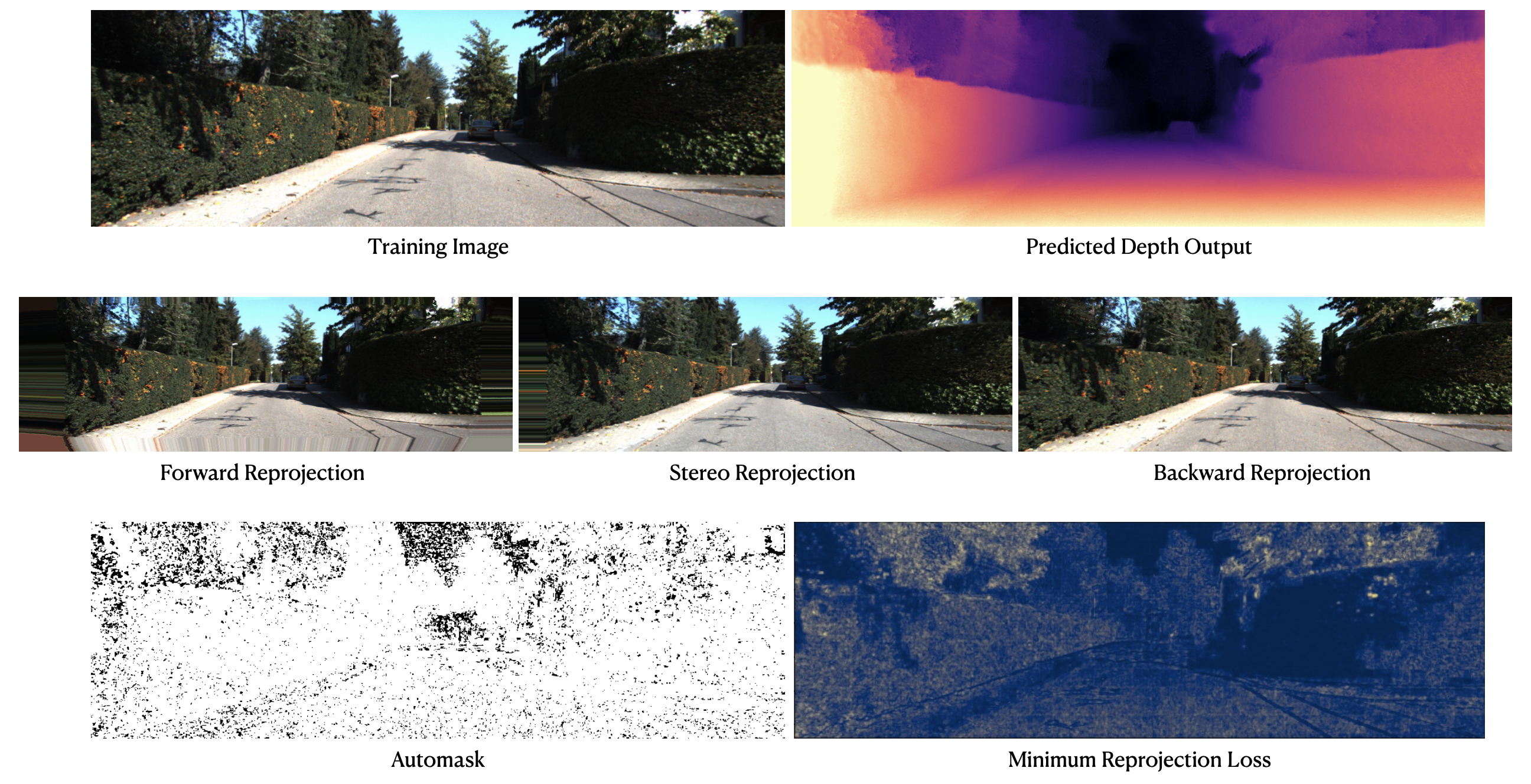
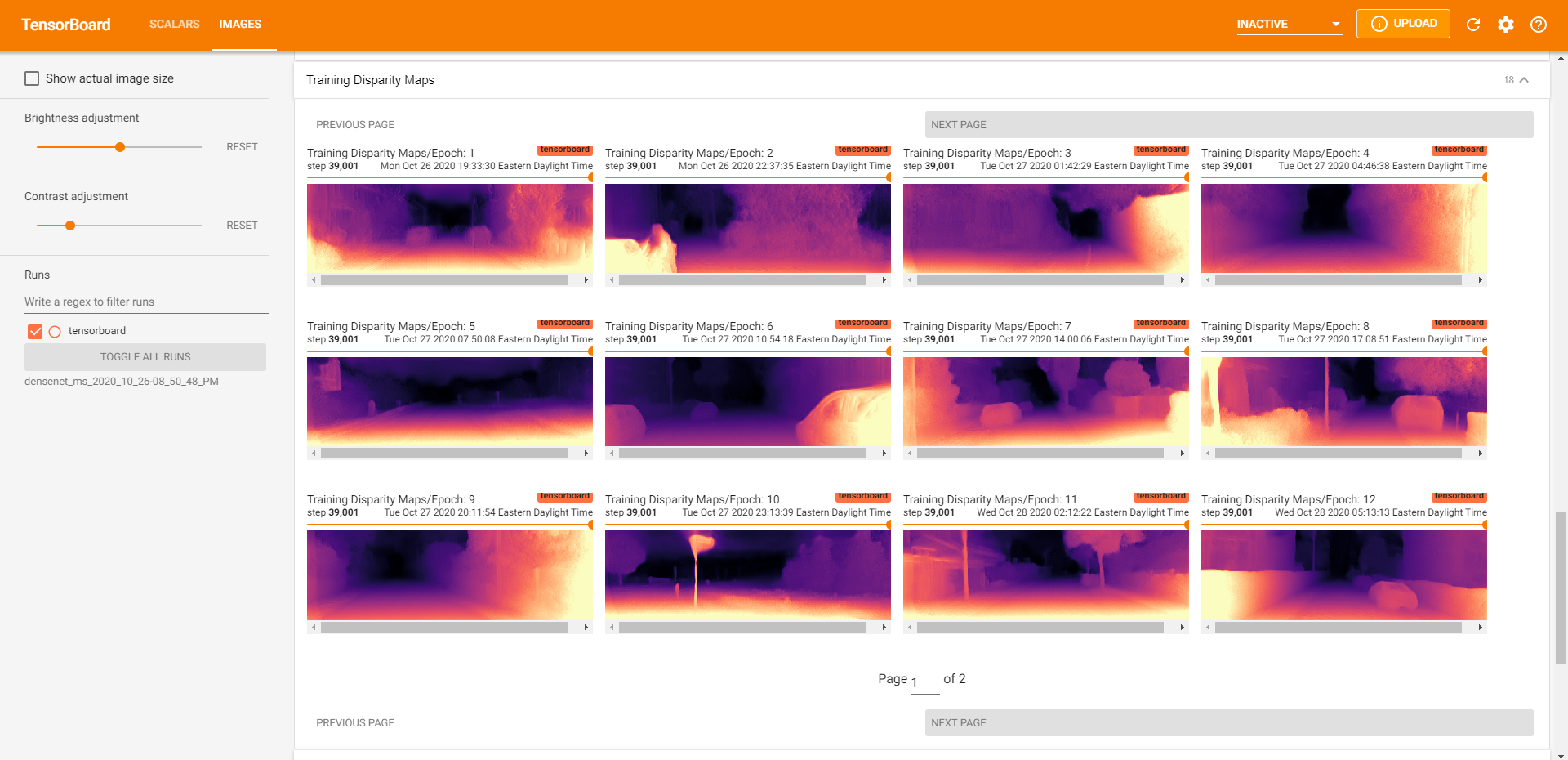
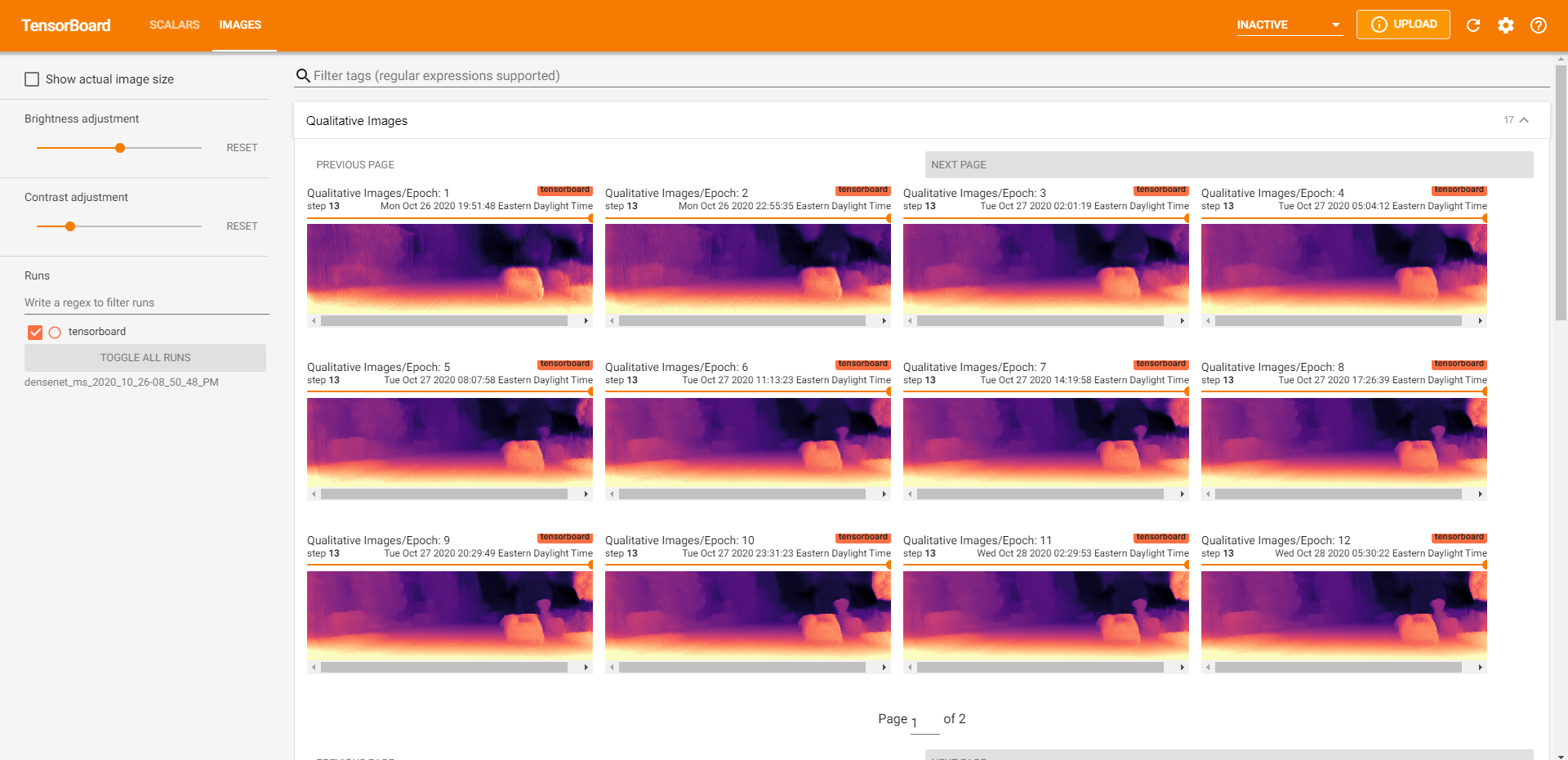
Our TensorBoard visualizations allow us to debug efficiently. We are able to quickly sanity check results by visualizing the predicted depth map, forward / backward / stereo reprojections, automasks, and losses.

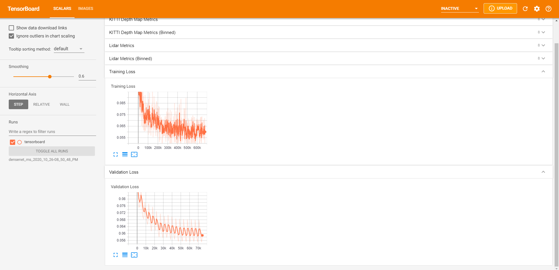
We display training / validation loss metrics and validation metrics to quickly monitor training jobs.

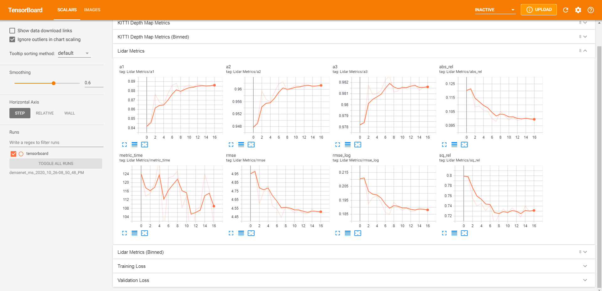
Loss figure Metrics figure over epochs

Additionally, we save the depth map results from each epoch to visualize how the model has changed over time across our manually curated dataset (~15 images). This also enables easy model comparison afterward (example above).

Training image disparity maps Chosen image disparity maps

Instructions

I do not include instructions for how to train or run the model on this page. However, if you wish to set up training or evaluation, you may check our GitHub repo or an adapted version of the README here.